Algebra

Finding the zeros of a polynomial from a graph

The zeros of a polynomial are the solutions to the equation p(x) = 0, where p(x) represents the polynomial. If we graph this polynomial as y = p(x), then you can see that these are the values of x where y = 0. In other words, they are the x-intercepts of the graph.

The zeros of a polynomial can be found by finding where the graph of the polynomial crosses or touches the x-axis.

[adsenseWide]

Let’s try this out with an example!

Example

Consider a polynomial f(x), which is graphed below. What are the zeros of this polynomial?

To answer this question, you want to find the x-intercepts. To find these, look for where the graph passes through the x-axis (the horizontal axis).

This shows that the zeros of the polynomial are: x = –4, 0, 3, and 7.

While here, all the zeros were represented by the graph actually crossing through the x-axis, this will not always be the case. Consider the following example to see how that may work.

Example

Find the zeros of the polynomial graphed below.

As before, we are looking for x-intercepts. But, these are any values where y = 0, and so it is possible that the graph just touches the x-axis at an x-intercept. That’s the case here!

From here we can see that the function has exactly one zero: x = –1.

Connection to factors

You may remember that solving an equation like f(x) = (x – 5)(x + 1) = 0 would result in the answers x = 5 and x = –1. This is an algebraic way to find the zeros of the function f(x). Each of the zeros correspond with a factor: x = 5 corresponds to the factor (x – 5) and x = –1 corresponds to the factor (x + 1).

So if we go back to the very first example polynomial, the zeros were: x = –4, 0, 3, 7. This tells us that we have the following factors:

(x + 4), x, (x – 3), (x –7)

However, without more analysis, we can’t say much more than that. For example, both of the following functions would have these factors:

f(x) = 2x(x+4)(x–3)(x–7)

and

g(x) = x(x+4)(x–3)(x–7)

In the second example, the only zero was x = –1. So, just from the zeros, we know that (x + 1) is a factor. If you have studied a lot of algebra, you recognize that the graph is a parabola and that it has the form $a(x+1)^2$ , where a > 0. But only knowing the zero wouldn’t give you that information*.

*you can actually tell from the graph AND the zero though. Since the graph doesn’t cross through the x-axis (only touches it), you can determine that the power on the factor is even. But, this is a little beyond what we are trying to learn in this guide!

Solving systems of equations by graphing

While systems of two linear equations with two unknowns can be solved using algebra, it is also possible to systems of equations by graphing each equation in the system. In the examples below, you will see how to find the solution to a system of equations from a graph, how to determine if there are no solutions, and how to determine if there are infinitely many solutions. You will also see an example of nonlinear systems and its graph.

[adsenseWide]

The graph of a system of equations with with one solution

Consider the following system of equations.

$\begin{array}{l} x+2y=8\\ \\x-2y=-4\end{array}$

If you solve this system using the addition method, you will find that $x = 2$ and $y = 3$. But, what does this look like on a graph?

solution-to-system-of-equations

Notice that the two lines intersect at exactly one point, and that this point is $(2, 3)$. For any system with one solution, the graphs will intersect at one point and this point will represent the solution to the system of equations.

If you don’t remember how to graph these equations, make sure to check this article: how to graph linear equations.

The graph of a system of equations with no solutions

The following system of equations has no solution.

$\begin{array}{l} x-y=-2\\ \\x-y=1\end{array}$

How would you know? One way would be to try and solve the system, and see that you get an untrue statement. Another would be to realize that the first equation is saying that x–y is one number, while the second equation is saying that x–y has a different value. These can’t both be true. The difference must have a single value.

You could also tell by looking at the graph of the system of equations.

no-solution-to-system-of-equations

The two lines are parallel, meaning that they will never intersect. For any system of equations, if there is no solution the the system, the two graphs will not intersect at any point. For linear equations, this will result in a graph of two parallel lines.

Infinitely many solutions.

Let’s look now at a system of equations with infinitely many solutions. While it will not always be so obvious, you can tell that this system has infinitely many solutions because the second equation is just a multiple of the first.

$\begin{array}{l} x+y=-2\\ \\2x+2y=-4\end{array}$

If you were to graph these two equations, you would get the following result.

infinitely-many-solutions

Even though the system of equations includes two linear equations, you end up with a single line. This will always be the case when there are infinitely many solutions. The solution set is actually all points along the line.

Can there be two or three or four solutions?

You may have noticed that we covered only three cases: one solution, no solutions, and infinitely many solutions. When working with linear equations, these are the only possibilities.

This is because the graphs of the equations are lines. A straight line can only intersect another straight line at one point, at no points, or at all points (they are just the same line). If two lines intersected at, say exactly two points, then the lines would have to bend and would no longer be lines.

If you are working with nonlinear equations, however, things are quite different! For example, in the graph below, the circle and the line intersect at exactly two points.

graph-of-system-of-equations-ex2

These two points would represent solutions to the system of equations. But again, this is only because both graphs are not from a linear equation.

Matrix notation and the size of a matrix

Matrices are used in a variety of different math settings from algebra and linear algebra to finite math. Of course, to be able to work with matrices, you need to understand the notation used and simple (but important) ideas like the size of a matrix.

[adsenseWide]

Elements of a matrix

A matrix is a way of organizing numbers into rows and columns. It may represent a system of equations, a real-life situation, or simply be a matrix of interest all on its own. Matrices are most commonly labeled with capital letters such as A, B, or C. Below, you can see a matrix we will refer to as “matrix A“.

example-of-a-matrix

The numbers within the matrix, are referred to as elements. One way to talk about a specific element is to use a lowercase letter and label it with the row and column of the element.

elements-of-a-matrix

Note that you could also say “5 is the (1,2) entry” and “8 is the (2,3) entry”.

The size of a matrix

The common theme with matrices is “think rows-columns”, and this holds even when discussing the size or dimension of a matrix. If a matrix has 4 rows and 6 columns, we say it is a 4 x 6 matrix (read: four by six).

size-of-a-matrix

Summary

As you study matrices, remember the following ideas:

Elements are referred to by their location in terms of the row, then column.
The size of a matrix is: (number of rows) x (number of columns). For a 2 x 3 matrix, you would say “the size of the matrix is 2 by 3”.

Continue studying matrices

Now that you have reviewed important notation and ideas like the size of a matrix, you are ready to study how to add, subtract, and multiply matrices.

Operations with matrices:

Adding and subtracting polynomials

As you will see below, in order to add or subtract polynomials, you really just need to pay attention to signs and combine like terms. This is especially important with subtraction, as you will be distributing a negative sign.

[adsenseWide]

Table of contents:

Adding polynomials
Subtracting polynomials

Adding polynomials

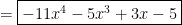
There are only really two steps required for adding two polynomials. For example, consider adding $x^2 + 4x + 1$ and $4x^2 - 2$ . In the picture, like terms are underlined the same number of times.

how-to-add-polynomials

For practice, let’s apply these steps to a couple more problems.

Example

Find the sum: $-3x^4 + 5x^3 - 7$ and $-8x^4 - 10x^3 + 3x + 2$

Remember here that “find the sum” is another way of saying “add”. So, we will first set up the addition and then combine like terms. Just as in the picture, like terms are underlined.

$(-3x^4 + 5x^3 - 7) + (-8x^4 - 10x^3 + 3x + 2)$

$= -\underline{3x^4} + \underline{\underline{5x^3}} - \underline{\underline{\underline{7}}} -\underline{8x^4} -\underline{\underline{ 10x^3}} + 3x + \underline{\underline{\underline{2}}}$

$= \boxed{-11x^4 -5x^3 + 3x -5}$

In some problems, you may find that the set up is already done. In these cases, you need only worry about combining like terms.

Example

Simplify: $(14y^3 + 2y^2) + (3y^3 + 7y^2)$

Although the instructions say simplify, you can see that this is actually a polynomial addition problem. Therefore, we can find the answer with the following steps.

$(14y^3 + 2y^2) + (3y^3 + 7y^2)$

$=\underline{14y^3} + \underline{\underline{2y^2}} + \underline{3y^3} + \underline{\underline{7y^2}}$

$=\boxed{17y^3 + 9y^2}$

Subtracting polynomials

When subtracting two polynomials, there is one extra step we must apply before combining like terms: distribute the negative. As an example, consider $(x^2 + 5) - (2x^2 -1)$ .

how-to-subtract-polynomials

Notice that when you distribute the negative, you distribute it to every term in the parentheses. Pay close attention to this in the next couple of examples.

Example

Find the difference: $(-4x^3 + x^2 - 1) - (-2x^3 + 3x^2 + 5)$

Just as “find the sum” means to add, “find the difference” means to subtract. Therefore, we will set up the subtraction, distribute the negative, and then collect like terms to find the answer.

$(-4x^3 + x^2 - 1) - (-2x^3 + 3x^2 + 5)$

$= -\underline{4x^3} + \underline{\underline{x^2}} - 1 + \underline{2x^3} - \underline{\underline{3x^2}} - 5$

$= \boxed{-2x^3 -2x^2 -6}$

As you can see, the main idea is to keep track of the signs. Also note, that just as with addition, instructions may just say “simplify”. Even so, you will still distribute the negative before combining like terms.

Example

Simplify: $(12x^5 -x) - (18x^5 + 4x^2 + x + 1)$

$=\underline{12x^5} -\underline{\underline{x}} - \underline{18x^5} - 4x^2 - \underline{\underline{x}} - 1$

$=\boxed{-6x^5 - 4x^2 - 2x - 1}$

Summary

Now that you have studied how to add and subtract polynomials, let’s review the overall steps.

Set up the addition or the subtraction.
Distribute the negative (if subtracting).
Combine like terms / simplify.

You will find later that these skills are important when working with rational expressions, long division of polynomials, and even when working with functions!

Understanding Exponents

When working with exponents, there are two new words that come up: exponent and base. As an example, in $x^2$, 2 is the exponent while $x$is the base and in $4^{12}$, 12 is the exponent while 4 is the base.

Table of contents:

Whole number exponents are about multiplication
Negative exponents
Fractions as exponents
Exponents on the calculator

[adsenseWide]

Whole number exponents are about multiplication

As long as the exponent is a positive whole number, you can think of it as telling you how many times you should multiply the base by itself.

$2^3=2\cdot2\cdot2=8$
$x^3=x\cdot x\cdot x$
$5^2=5\cdot5=25$

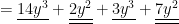
As you can see, $4^{12}$ means “4 multiplied by itself 12 times” and that is a really big number. Many values that you calculate from exponents will be quite large.

There are a couple of things to note:

Anything with an exponent of zero is defined to be 1. So, $4^{0}=1$, $100^{0}=1$.
Ok right above, when I said anything, I meant “almost anything”. $0^0$ is an indeterminate form. For everything else however, the rule above holds.
An exponent of 1 is the same as just writing the number by itself: $4^{1}=4$.

Negative Exponents

Negative exponents are treated a bit differently. By definition, if we have a positive number $n$ and a nonzero $b$, then the following rule holds:

$b^{-n} = \frac{1}{b^n}$

Using this rule, if you see a value with a negative exponent, then it can be rewritten as 1 “over” that term with a positive exponent. Here are a few examples of how this works.

$3^{-2} = \frac{1}{3^2} = \frac{1}{9}$

$10^{-1} = \frac{1}{10^1} = \frac{1}{10}$

$(-2)^{-4} = \frac{1}{(-2)^4} = \frac{1}{16}$

As you can see, it is simply about following the formula when dealing with negative exponents. After this, you can simply calculate the value using the rules above.

Fractions as exponents

In algebra and more advanced math, it is very common to see an exponent of one-half or some other fraction. This is one way to represent terms involving roots, or radical terms. By definition (if n is nonzero):

$b^{\frac{m}{n}}= \sqrt[n]{b^m}$

Working with these types of terms (radical terms) is a more advanced topic and will be the subject of a different article, but it is important that you be able to rewrite such terms using the definition as below.

$3^{\frac{1}{2}}=\sqrt{3^1}=\sqrt{3}$

$4^{\frac{2}{3}}=\sqrt[3]{4^2} = \sqrt[3]{16}$

As you study terms involving exponents, you will find that you need to combine rules quite often. For example, the rule above can be combined with the rule for negative exponents to simplify even more complex expressions.

Using a Calculator

Finding the value of terms with exponents on scientific or graphing calculators is quite easy. The usual key you will need will use a carat symbol ^ to represent that the next number is an exponent. So, $3^4$ can be represented as 3^4 in most calculators. On the TI83 or TI84:

screenshot-exponent-calculator

You can also always use the carat symbol on google (just type it into google! they now do automatic calculations for you) or wolfram alpha.

[adsenseLargeRectangle]

Additional Reading

As you continue studying exponents, you will also want to review the order of operations. This lesson will show you how to handle expressions that have exponents, multiplication, and other operations all together.

Understanding and finding y-intercepts

The y-intercept of a graph is the point where it crosses the y-axis, which is the vertical axis from the xy-coordinate plane. Below, we will see how to find the y-intercept of any function and why a function can have at most one y-intercept in general. You can also always scroll down to a video example.

[adsenseWide]

Seeing it on a graph

Before we go into detail, consider the graph below. As you can see, it is a linear function (the graph is a line) and it crosses the y-axis at the point (0, 3). This tells you that the y-intercept is 3.

graph showing line crossing y-axis at the point (0,3)

Since any point along the y-axis has an x-coordinate of 0, the form of any y-intercept is $(0, c)$ for some number $c$.

Using algebra to find the y-intercept of a function

To find the y-intercept of a function, let $x = 0$ and solve for $y$. Consider the following example.

Example

Find the y-intercept of the function: $y = x^2 + 4x – 1$

Solution

Let $x = 0$ and solve for $y$.

$\begin{align} y &= 0^2 + 4(0) – 1\\ &= \boxed{-1}\end{align}$

Thus the y-intercept is –1 and is located at the point $(0, –1)$.

A closer look

Now that we have seen how to find them, there are two interesting questions that can come up:

Can a function have more than one y intercept?
Can a function have no y intercept?

In answering these, remember that by definition, a function can only have one output (y-value) for each input (x-value). A function having more than one y-intercept would violate this, since it would mean that there are two outputs for $x = 0$. Therefore, it is not possible for a function to have more than one y-intercept.

What about no y intercept? Well, consider the graph below. This is a graph of the function: $y = \dfrac{1}{x}$

a graph of y = 1/x, which has no y-intercept

This function never crosses the y-axis because, since you can’t divide by zero, it is undefined at $x = 0$. In fact, any time a function is undefined at 0, it will have no y-intercept.

Video example

In the video below, I show you three examples of how to find the y-intercept. As you will see, the idea is pretty straight-forward!

Summary

When working with any graph, two useful things to know are the location of any x-intercepts, and the location of the y-intercept, if it exists. With a linear function (a line) these two points are enough to quickly sketch a graph. For more complex functions however, finding intercepts is often part of a deeper analysis.

[adsenseLargeRectangle]

Continue your study of graphing

You may find the following articles useful as you continue to study graphs:

Finding and understanding x-intercepts

Finding and understanding x-intercepts

Given the graph of any function, an x-intercept is simply the point, or points where the graph crosses the x-axis. There might be just one such point, no such point, or many, meaning a function can have several x-intercepts. As you will see below, we can use a graph or a simple algebra rule to find the x-intercept or x-intercepts of any function. You can also scroll down to a video example below.

Table of Contents

Using a graph to find x-intercepts
Using algebra to find x-intercepts
Video example (including when there are no x-intercepts)
Further reading

[adsenseWide]

Finding the x-intercept or x-intercepts using a graph

As mentioned above, functions may have one, zero, or even many x-intercepts. These can be found by looking at where the graph of a function crosses the x-axis, which is the horizontal axis in the xy-coordinate plane. You can see this on the graph below. This function has a single x-intercept.

a graph with an x-intercept of 2

In the graph below, the function has two x-intercepts. Notice that the form of the point is always $(c, 0)$ for some number $c$.

Graph showing a function with two x-intercepts. The graph crosses the x-axis two times.

Finally, the following graph shows a function with no x-intercepts. You can see this because it does not cross the x-axis at any point.

Graph showing a function with no x-intercepts. The function's graph does not cross the x-axis.

You can see a more advanced discussion of these ideas here: The zeros of a polynomial.

Finding the x-intercept or intercepts using algebra

The general rule for finding the x-intercept or intercepts of any function is to let $y = 0$ and solve for $x$. This may be somewhat easy or really difficult, depending on the function. Let’s look at some examples to see why this may be the case.

Example

Find the x-intercept of the function: $y = 3x – 9$

Solution

Let $y = 0$ and solve for $x$.

$\begin{align}0 &= 3x – 9\\ -3x &= -9\\x &= 3\end{align}$

Answer: Therefore the x-intercept is 3. You could also write it as a point: $(3,0)$

A more complicated example would be one where the equation representing the function itself is more complex. For these situations, you need to know a little more algebra in order to find any intercepts.

Example

Find the x-intercepts for the function: $y = x^2 + 2x – 8$

Solution

As before, let $y = 0$ and solve for $x$. This time, you have a quadratic equation to solve.

$\begin{align} 0 &= x^2 + 2x – 8\\ 0 &= (x + 4)(x – 2)\\ x &= -4, 2\end{align}$

Answer: This function has two x-intercepts: –4 and 2. These are located at $(–4, 0)$ and $(2, 0)$.

For equations more complex than this, a graphing calculator is often useful for at least estimating the location of any intercepts.

[adsenseLargeRectangle]

Video examples

In the following video, you can see how to find the x-intercepts of three different functions. This also includes an example where there are no x-intercepts.

Continue your study of graphs

You can continue your study of graphing with the following articles.

Finding y-intercepts

Visualizing Matrix Multiplication

Matrix multiplication is just one of those things that is not intuitive – at least not at first. You have just had so many years of multiplication meaning one thing and then you have this entirely new definition to work with! It certainly takes some getting used to. (and if you continue to study advanced math – get used to that idea of “getting used to” things)

The easiest way to think of it is “rows hit columns and fill up rows”. This process is repeated until you run out of rows in the first matrix. This is seen in the following animation (no sound).

You can read more about how to multiply matrices here, including examples and important properties: Multiplying matrices.

Sketching Quick and Accurate Graphs of Linear Equations

While there are plenty of methods to get a good hand drawn graph of a linear equation, many plot more points than necessary and (if you aren’t careful) misrepresent the location of two important points: the x and y intercepts.

Using the intercepts to plot your line takes care of both of these problems and more importantly: its fast! In this video, I will use two examples to show you exactly how it’s done.

[flv]http://www.mathbootcamps.com/media/fastgraphsoflinearequations.mp4[/flv]

Why can’t you cancel the x?

Without even writing down any algebra, you probably already know what types of problems this article is talking about. There are problems that come up in algebra where it seems like you should be able to cancel a variable out and move on. Yet, in these very situations your professor or teacher keeps telling you it can’t happen. Why is this the case?

Below, we will look at some specific examples and see the difference between when you can cancel a variable and when you can’t.

[adsenseWide]

It is all about factors

It may not always seem like it, but there really is a pattern and a simple rule of when you can and can’t cancel a term or a variable. Let’s focus on rational expressions specifically. Those are expressions (like the one below) where both the numerator and the denominator are polynomials. An example is:

$\dfrac{x+5}{x^2+1}$

When can you cancel terms in a rational expression?

You can cancel any matching factors that occur in both the numerator and the denominator. Let’s use numbers to understand this a little better. Consider the fraction below:

$\dfrac{4}{14}$

In the fraction above, 2 is a factor of 4 since $2 \times 2 = 4$. Similarly, 2 is a factor of 14 since $2 \times 7 = 14$. Based on the rule of cancelling common factors, we should be able to cancel the 2’s and get a fraction that has the same value.

$\dfrac{4}{14}=\dfrac{2(2)}{2(7)}=\dfrac{2}{7}$

If you check on a calculator you will find that 4 divided by 14 is the same as 2 divided by 7 – so this rule seems to be working here. What is really going on?

Why does this work?

Every number other than zero, when divided by itself is 1. Since a fraction simply represents division (in one sense), $\dfrac{2}{2} = 1$ and we really just have $1\times\dfrac{2}{7}$.

Trying it with Variables

Now that everything makes some sense with numbers, let’s try variables.You can think of it as though the variables represent numbers, so they will behave in the same way. Take for instance the expression below.

$\dfrac{x^2-x}{x^3}, x\neq 0$

The numerator has a couple of factors which we can find by factoring out an $x$:

$x^2-x = x(x-1)$

This shows us that $x$ and $x-1$ are factors of the numerator. Looking at the denominator, we see $x$ is also a factor since $x^3=x(x^2)$. Remember, when both the numerator and the denominator share a factor, you can cancel that factor from the fraction. This means that we can simplify the original rational expression:

$\begin{align} \dfrac{x^2-x}{x^3} &= \\ \dfrac{x(x^2-1)}{x(x^2)} &= \boxed{\dfrac{x^2-1}{x^2}}\end{align}$

The only time you can’t cancel terms in the numerator and denominator is when they are both NOT factors.. That’s why you can’t cancel $x$ in $\dfrac{x-5}{x}$. The $x$ is not a factor of the numerator; its just a term being added. Cancelling the $x$ here would be like cancelling the $5$ in $\dfrac{5+1}{5}$ and saying that is 1, when really $\dfrac{5+1}{5}$ = \dfrac{6}{5}. This is certainly not equivalent to one!

[adsenseLargeRectangle]

Summary

Simplifying rational expressions, like those seen above, requires the same skills you used when simplifying fractions like $\dfrac{2}{4}$ or $\dfrac{8}{10}$. You are always looking for common factors. If $x$ or whatever expression you are looking at isn’t a common factor of the numerator and denominator, then you can’t cancel it out of the rational expression.